How Does Triangle Inequality Change Tsp Problem

Open up admission peer-reviewed chapter

How to Solve the Traveling Salesman Problem

Submitted: September 23rd, 2020 Reviewed: January 20th, 2021 Published: February 9th, 2021

DOI: ten.5772/intechopen.96129

IntechOpen Downloads

393

Full Chapter Downloads on intechopen.com

Abstract

The Traveling Salesman Problem (TSP) is believed to be an intractable problem and have no practically efficient algorithm to solve it. The intrinsic difficulty of the TSP is associated with the combinatorial explosion of potential solutions in the solution space. When a TSP instance is big, the number of possible solutions in the solution space is so large equally to forbid an exhaustive search for the optimal solutions. The seemingly "limitless" increase of computational power will non resolve its genuine intractability. Do we demand to explore all the possibilities in the solution space to notice the optimal solutions? This chapter offers a novel perspective trying to overcome the combinatorial complexity of the TSP. When we pattern an algorithm to solve an optimization problem, we usually enquire the critical question: "How tin can we discover all exact optimal solutions and how do nosotros know that they are optimal in the solution infinite?" This chapter introduces the Attractor-Based Search System (ABSS) that is specifically designed for the TSP. This affiliate explains how the ABSS answer this critical question. The calculating complexity of the ABSS is also discussed.

Keywords

• combinatorial optimization
• global optimization
• heuristic local search
• computational complication
• traveling salesman problem
• multimodal optimization
• dynamical systems
• attractor

• Weiqi Li*

  • School of Management, University of Michigan-Flint, Flintstone, USA

*Address all correspondence to: weli@umich.edu

i. Introduction

The TSP is one of the nearly intensively investigated optimization bug and oft treated as the prototypical combinatorial optimization trouble that has provided much motivation for design of new search algorithms, development of complexity theory, and analysis of solution space and search space [1, 2]. The TSP is defined as a complete graph Q = V E C , where Five = v i : i = one two … n is a ready of northward nodes, Eastward = e i j : i j = ane two … n i ≠ j northward × n is an edge matrix containing the set of edges that connects the due north nodes, and C = c i j : i j = i 2 … n i ≠ j northward × n is a cost matrix belongings a set of traveling costs associated with the set of edges. The solution space South contains a finite set of all viable tours that a salesman may traverse. A tour s ∈ Southward is a closed route that visits every node exactly one time and returns to the starting node at the finish. Like many existent-world optimization issues, the TSP is inherently multimodal; that is, it may contain multiple optimal tours in its solution space. We presume that a TSP instance Q contains h ≥ i optimal tours in S . Nosotros announce f ( southward ) equally the objective function, s ∗ = min due south ∈ Southward f s every bit an optimal bout and South ∗ every bit the set of h optimal tours. The objective of the TSP is to find all h optimal tours in the solution space, that is, S ∗ ⊂ S . Therefore, the argument is

arg min s ∈ S f s = S ∗ = s 1 ∗ s ii ∗ … s h ∗

E1

Under this definition, the salesman wants to know what all best alternative tours are available. Finding all optimal solutions is the essential requirement for an optimization search algorithm. In practice, cognition of multiple optimal solutions is extremely helpful, providing the decision-maker with multiple options, particularly when the sensitivity of the objective function to pocket-size changes in its variables may be different at the alternative optimal points. Manifestly, this TSP definition is elegantly elementary only full of claiming to the optimization researchers and practitioners.

Optimization has been a fundamental tool in all scientific and engineering areas. The goal of optimization is to find the all-time set of the admissible conditions to accomplish our objective in our decision-making process. Therefore, the fundamental requirement for an optimization search algorithm is to find all optimal solutions within a reasonable corporeality of computing time . The focus of computational complexity theory is to analyze the intrinsic difficulty of an optimization problem and the asymptotic property of a search algorithm to solve information technology. The complexity theory attempts to address this question: "How efficient is a search algorithm for a particular optimization problem, as the number of variables gets large?"

The TSP is known to be NP-hard [2, 3]. The problems in NP-difficult class are said to be intractable because these bug have no asymptotically efficient algorithm, fifty-fifty the seemingly "limitless" increase of computational power will not resolve their genuine intractability. The intrinsic difficulty of the TSP is that the solution space increases exponentially every bit the trouble size increases, which makes the exhaustive search infeasible. When a TSP example is big, the number of possible tours in the solution space is so big to forbid an exhaustive search for the optimal tours. A viable search algorithm for the TSP is one that comes with a guarantee to find all best tours in time at most proportional to n k for some power grand .

Do we demand to explore all the possibilities in the solution space to find the optimal solutions? Imagine that searching for the optimal solution in the solution space is similar treasure hunting. We are trying to hunt for a hidden treasure in the whole globe. If we are "blindfolded" without any guidance, information technology is a silly idea to search every single square inch of the extremely large space. Nosotros may take to perform a random search procedure, which is usually non effective. However, if nosotros are able to use various clues to locate the pocket-sized village where the treasure was placed, we will then directly go to that village and search every corner of the hamlet to find the hidden treasure. The philosophy backside this treasure-hunting case for optimization is that: if we practice not know where the optimal signal is in the solution infinite, nosotros tin can attempt to identify the small region that contains the optimal point and then search that small-scale region thoroughly to notice that optimal point.

Optimization researchers take developed many optimization algorithms to solve the TSP. Deterministic approaches such equally exhaustive enumeration and branch-and-jump can find verbal optimal solutions, but they are very expensive from the computational point of view. Stochastic optimization algorithms, such as simple heuristic local search, Evolutionary Algorithms, Particle Swarm Optimization and many other metaheuristics, tin find hopefully a good solution to the TSP [ane, four, 5, six, seven]. The stochastic search algorithms merchandise in guaranteed definiteness of the optimal solution for a shorter computing fourth dimension. In practice, virtually stochastic search algorithms are based on the heuristic local search technique [eight]. Heuristics are functions that help us decide which ane of a ready of possible solutions is to be selected next [9]. A local search algorithm iteratively explores the neighborhoods of solutions trying to improve the current solution past a local change. However, the scope of local search is limited by the neighborhood definition. Therefore, heuristic local search algorithms are locally convergent. The final solution may deviate from the optimal solution. Such a final solution is called a locally optimal solution , denoted as south ′ in this affiliate. To distinguish from locally optimal solutions, the optimal solution s ∗ in the solution space is usually called the globally optimal solution .

This chapter studies the TSP from a novel perspective and presents a new search algorithm for the TSP. This affiliate is organized in the following sections. Section 2 presents the ABSS algorithm for the TSP. Section three describes the important data construction that is a critical player in solving the TSP. Section 4 discusses the nature of heuristic local search algorithm and introduces the concept of solution attractor. Section 5 describes the global optimization features of the ABSS. Section 6 discusses the computational complexity of the ABSS. Section 7 concludes this affiliate.

Advertizement

2. The attractor-based search organisation for the TSP

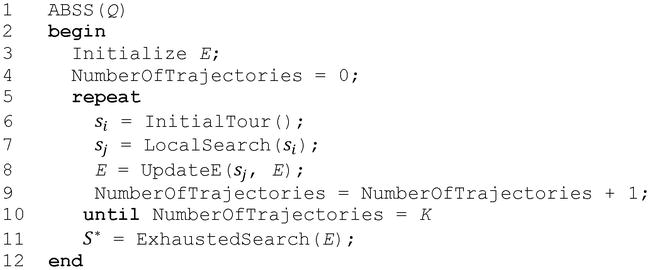
Figure one presents the Attractor-Based Search Organization (ABSS) for the TSP. In this algorithm, Q is a TSP instance with the edge matrix Eastward and cost matrix C . At commencement of search, the matrix E is initialized by assigning zeros to all elements of E . The roleInitialTour()constructs an initial bout south i using any bout-construction technique. The officeLocalSearch()takes southward i as an input, performs local search using whatever type of local search technique, and returns a locally optimal tour due south j . The functionUpdateE()updates the matrix E by recording the edge configuration of tour south j into the matrix. K is the number of search trajectories. After the edge configurations of One thousand locally optimal tours are stored in the matrix Due east , the functionExhaustedSearch()searches E completely using the depth-first tree search technique, which is a elementary recursive search method that traverses a directed graph starting from a node then searches adjacent nodes recursively. Finally, the ABSS outputs a set of all best tours S ∗ found in the edge configuration of E . The search strategy in the ABSS is straightforward: generating Yard locally optimal tours, storing their edge configurations in the matrix East , and so identifying the best tours by evaluating all tours represented by the border configuration of E . The ABSS is a simple and efficient reckoner program that can solve the TSP effectively. This search algorithm shows potent features of effectiveness, flexibility, adaptability, scalability and efficiency. The computational model of the ABSS is inherently parallel, facilitating implementation on concurrent processors. It can be implemented in many unlike means: serial, parallel, distributed, or hybrid.

Figure 1.

The ABSS algorithm for the TSP.

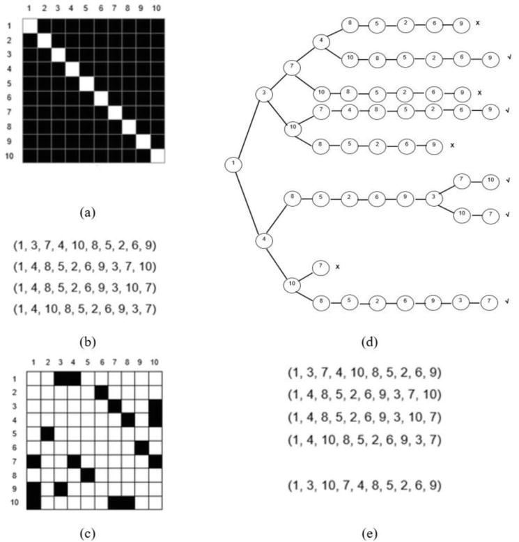
Figure 2 uses a 10-node instance as an example to illustrate how the ABSS works. We randomly generate Chiliad = 6 due north = sixty initial tours, which edge configurations hit all elements of the matrix Eastward (marked as black color), as shown in Figure ii(a). Information technology means that these lx random tours hit all 45 edges that correspond all 181440 tours in the solution space. We let each of the search trajectories run 5000 iterations and obtain 60 locally optimal tours. However, due to the small size of the instance, about locally optimal tours have identical edge configurations. Amid the 60 locally optimal tours, nosotros detect merely four singled-out locally optimal tours as shown in Figure 2(b). Figure 2(c) shows the union of the edge configurations of the 60 locally optimal tours, in which 18 edges are hit. So we use the depth-offset tree search, as illustrated in Figure 2(d), to identify all five tours in the edge configuration of E , which are listed in Effigy two(due east). In fact, one of the five tours is the globally optimal tour. This simple example indicates that (i) local search trajectories converge to pocket-sized fix of edges, and (2) the union of the edge configurations of K locally optimal tours is not but a countable marriage of the edge configurations of the these tours, only also include the border configurations of other locally optimal tours. The ABSS consists of two search phases: local search phase and exhaustive search phase. The job of the local search phase is to identify the region that globally optimal tour is located (i.e. the village hiding the treasure), and the task of the exhaustive search phase is to observe the globally optimal tour (i.e. find the hidden treasure). The remaining sections will briefly explain the features of the ABSS.

Figure 2.

A simple instance of the ABSS algorithm. (a) Matrimony of the edge configurations of lx random initial tours, (b) four distinct locally optimal tours, (c) union of the edge configurations of the 60 locally optimal tours, (d) the depth-kickoff tree search on the edge configuration ofE, and (e) v tours found inDue east.

In all experiments mentioned in the affiliate, we generate symmetric TSP instances with n nodes. The chemical element c i j of the cost matrix C is assigned a random integer independently fatigued from a uniform distribution of the range [ane, 1000]. The triangle inequality c i j + c j thousand ≥ c i m is not assumed in the instances. Although this type of problem instances is application-costless, it is mathematically significant. A TSP instance without triangle inequality cannot exist approximated within any constant gene. A heuristic local search algorithm ordinarily performs much worse for this type of TSP instances, which offers a strikingly challenge to solving them [2, 3, 6, 10, 11]. We apply the 2-opt local search technique in the local search phase. The 2-opt neighborhood can be characterized as the neighborhood that induces the greatest correlation between role values of neighboring tours, because neighboring tours differ in the minimum possible 4 edges. Forth the same reasoning line, the two-opt may take the smallest expected number of locally optimal points [12]. The local search procedure randomly selects a solution in the neighborhood of the electric current solution. A move that gives the first improvement is called. The great advantage of the first-improvement pivoting rule is to produce randomized locally optimal points. The software program written for the experiments employ several unlike programming languages and are run in PCs with different versions of Window operating system.

Advertising

3. The border matrix E

Unremarkably the edge matrix E is not necessary to be included in the TSP definition because the TSP is a complete graph. However, the edge matrix Due east is an effective data structure that tin help usa sympathise the search behavior of a local search arrangement. Full general local search algorithm may not require much trouble-specific noesis in guild to generate good solutions. Nonetheless, it may be unreasonable to expect a search algorithm to be able to solve whatever problem without taking into account the data structure and properties of the problem at hand.

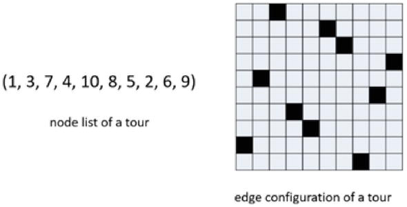
To solve a trouble, the offset pace is to create a manipulatable description of the trouble itself. For many issues, the pick of data structure for representing a solution plays a critical role in the assay of search beliefs and design of new search algorithm. For the TSP, a tour tin exist represented past an ordered list of nodes or an edge configuration of a tour in the edge matrix E , as illustrated in Figure 3. The comeback of the current tour represents the change in the order of the nodes or the edge configuration of a tour.

Figure three.

Two representations of a tour: an ordered list of nodes and an border configuration of a bout.

Observing the behavior of search trajectories in a local search organization can be quite challenging. The edge matrix E is a natural data structure that can assist u.s. trace the search trajectories and understand the dynamics of a local search system. An edge e i j is the near bones element of a bout, only contains a piece of information about each of northward − 2 ! tours that go through it. Essentially, the nature of local search for the TSP is an edge-choice process: preservation of skilful edges and rejection of bad edges according to the objective function f due south . Each edge has an implicit probability to exist selected by a locally optimal tour. A ameliorate edge has higher probability to be included in a locally optimal bout. Therefore, the edges in East can exist divided into 3 groups: globally superior edges, G -edges, and bad edges. A globally superior edge is the border that occurs in many or all locally optimal tours. Although each of these locally optimal tours selects this edge based on its own search trajectory, the edge is globally superior since the edge is selected by these individual tours from different search trajectories going through dissimilar search regions. The globally superior edges have higher probability to be selected past a locally optimal tour. A G -edge is the edge that is included in a globally optimal tour. All K -edges are globally superior edges and tin can be treated as a special subset of the globally superior edges. The edges that are discarded past all search trajectories or selected by only few locally optimal tours are bad edges. A bad border is impossible to be included in a globally optimal tour. A locally optimal tour usually consists of some G -edges, some globally superior edges and a few bad edges.

The changes of the edge configuration of the matrix E represent the transformations of the search trajectories in a local search system. When all search trajectories reach their end points, the final border configuration of Due east represents the final state of the local search system. For a bout due south yard , we define an element e i j of Due east every bit

e i j = 1 if the element e i j is in the tour s thousand 0 otherwise

E2

Then the hit-frequency value e ij in the element e i j is defined as the number of occurrence of the chemical element in K tours, that is

When Yard search trajectories accomplish their cease points, the value e ij + eastward ji / One thousand can represent the probability of the edge e i j being hit by a locally optimal tour. We can use graphical technique to notice the convergent behavior of the search trajectories through the matrix E . The hitting-frequency value e ij can be easily converted into a unit of measurement of one-half-tone information in a estimator, a value that we interpret every bit a number H ij somewhere between 0 and 1. The value 1 corresponds to black color, 0 to white color, and whatsoever value in between to a greyness level. Allow Yard be the number of search trajectories, the half-tone information H ij on a figurer screen tin can exist represented by the hit-frequency east ij in the chemical element due east i j of Due east :

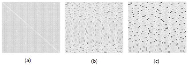
Effigy 4 illustrates a simple example of visualization showing the convergent behavior of 100 search trajectories for a l-node case. Effigy iv(a) shows the epitome of the edge configurations of 100 random initial tours. Since each element of E has equal chance to exist striking by these initial tours, nigh all elements are hitting past these initial tours, and all elements have very depression H ij values, ranging from 0.00 to 0.02. When the local search system starts searching, the search trajectories constantly change their edge configurations, and therefore the colors in the elements of Due east are changed accordingly. Every bit the search continues, more than and more elements become white (i.due east. they are discarded by all search trajectories) and other elements become darker (i.eastward. they are selected past more than search trajectories). When all search trajectories attain their end points, the colored elements represent the last border configuration of the search system. Effigy 4(b) and (c) show the images of edge configuration of E when all search trajectories completed 2000 iterations and 5000 iterations, respectively. At 5000th iteration, the range of H ij values in the elements of E is from 0.00 to 0.42. The value 0.42 means that 42% of the search trajectories select this element. Majority of the elements of E become white color.

Effigy four.

Visualization of the convergent dynamics of local search system. (a) the paradigm of the edge configurations of 100 initial tours, (b) and (c) the images of edge configurations when the search trajectories are at 2000th and 5000th iteration, respectively.

This simple example has smashing explanatory power about the global dynamics of the local search system for the TSP. As search trajectories continue searching, the number of edges hitting past them becomes smaller and smaller, and better edges are hit by more and more than search trajectories. This edge-convergence miracle means that all search trajectories are moving closer and closer to each other, and their edge configurations get increasingly similar. This phenomenon describes the globally asymptotic behavior of the local search arrangement.

Information technology is easily verified that under sure conditons, a local search system is able to notice the fix of the globally optimal tours S ∗ when the number of search trajectories is unlimited, i.due east.

However, the required search attempt may be very huge – equivalent to enumerating all tours in the solution infinite. Now 1 question for the ABSS is "How many search trajectories in the search organization practice we need to find all globally optimal tours?" The matrix E consists of n n − 1 elements (excluding the diagonal elements). When we randomly construct a bout and record its edge configuration in E , n elements of Eastward volition be hitting by this bout. If we construct more random tours and record their border configurations in E , more elements will be striking. We define Grand every bit the number of randomly-constructed initial tours, whose border configurations together will hit all elements of E . We know that all elements of Eastward represent all combinatorial possibilities in the solution space. Therefore, K is the number of search trajectories such that the union of edge configurations of ther initial tours covers the entire solution space. In our experiments, we constitute that the edge configurations of at well-nigh half-dozen n randomly-constructed tours can guarantee to hit all elements of E . From the tour perspective, Chiliad = 6 n random tours represent only a small set of the tours in the solution space. Nevertheless, from the view of edge-configuration, the marriage of the edge configurations of six n random tours represents the edge configurations of all tours in the solution infinite. It reveals an astonishing fact: the spousal relationship of the edge configurations of only vi n random tours contains the edge configurations of all n north − 1 ! / two tours in the solution space. It reflects the combinatorial nature of the TSP: the tours in the solution space are formed by different combinations of the edges. The union of the border configurations of a fix of tours contains information about many other tours because i bout shares its edges with many other tours. One cardinal theory that can help us explicate this miracle is the data theory [13]. According to the information theory, each solution point contains some information well-nigh its neighboring solutions that can be modeled as a role, chosen information function or influence function . The influence function of the i thursday solution point in the solution space S is defined as a part Ω i : S → R , such that Ω i is a decreasing office of the distance from a solution indicate to the i thursday solution indicate. The notion of influence office has been extensively used in datamining, data clustering, and pattern recognition.

Advertisement

four. The nature of heuristic local search

Heuristic local search is based on the concept of neighborhood search. A neighborhood of a solution southward i , denoted as North southward i , is a set of solutions that are in some sense close to s i . For the TSP, a neighborhood of a tour southward i is defined every bit a set of tours that can be reached from s i in one unmarried transition. From border-configuration perspective, all tours in N s i are very similar considering they share significant number of edges with due south i . The basic operation of local search is iterative improvement, which starts with an initial tour and searches the neighborhood of the electric current tour for a better tour. If such a tour is found, it replaces the current tour and the search continues until no improvement can be made. The local search algorithm returns a locally optimal bout.

The behavior of a local search trajectory can be understood as a process of iterating a search role grand due south . We denote s 0 as an initial indicate of search and thousand t s as the t th iteration of the search function g s . A search trajectory southward 0 , g s 0 , grand 2 s 0 , … , g t s 0 , … converges to a locally optimal point s ′ as its limit, that is,

thou lim t → ∞ g t south 0 = lim t → ∞ g t + 1 southward 0 = due south ′

E6

Therefore, a search trajectory will reach an terminate point (a locally optimal betoken) and will stays at this bespeak forever.

In a heuristic local search algorithm, there is a great variety of ways to construct initial bout, cull candidate moves, and define criteria for accepting candidate moves. About heuristic local search algorithms are based on randomization. In this sense, a heuristic local search algoorithm is a randomized organisation. There are no 2 search trajectories that are exactly alike in such a search arrangement. Different search trajectories explore different regions of the solution space and stop at different terminal points. Therefore, local optimality depends on the initial points, the neighborhood role, randomness in the search process, and time spent on search process. On the other hand, however, a local search algorithm essentially is deterministic and not random in nature. If we observe the motion of all search trajectories, we volition come across that the search trajectories become towards the same direction, move closer to each other, and eventually converge into a small-scale region in the solution infinite.

Heuristic local search algorithms are essentially in the domain of dynamical systems. A heuristic local search algorithm is a discrete dynamical system, which has a solution infinite S (the country space), a set up of times T (search iterations), and a search function g : South × T → S that gives the consequents to a solution south ∈ S in the form of southward t + 1 = yard s t . A search trajectory is the sequence of states of a single search procedure at successive time-steps, which represents the part of the solution infinite searched by this search trajectory. The questions about the behavior of a local search system over fourth dimension are actually the questions near its search trajectories. The most basic question most the search trajectories is "Where practise they get in the solution space and what do they do when they become there?"

The attractor theory of dynamical systems is a natural paradigm that can be used to describe the search behavior of a heuristic local search system. The theory of dynamical systems is an extremely broad surface area of written report. A dynamical organization is a model of describing the temporal evolution of a system in its state space. The goal of dynamical system assay is to capture the distinctive properties of certain points or regions in the state space of a given dynamical system. The theory of dynamical systems has discovered that many dynamical systems exhibt attracting behavior in the land space [fourteen, fifteen, xvi, 17, 18, 19, 20, 21, 22]. In such a arrangement, all initial states tend to evolve towards a single concluding point or a set of points. The term attractor is used to describe this unmarried point or the set of points in the state space. The attractor theory of dynamical systems describes the asymptotic beliefs of typical trajectories in the dynamical arrangement. Therefore, the attractor theory provides the theoretical foundation to study the search behavior of a heuristic lcoal search system.

In a local search organisation for the TSP, no matter where we start a search trajectory in the solution space, all search trajectories will converge to a small region in the solution space for a unimodal TSP example or h small regions for a h -model TSP. We call this small region a solution attractor of the local search system for a given TSP instance, denoted as A . Therefore, the solution attractor of a local search organization for the TSP can be defined every bit an invariant set A ⊂ S consisting of all locally optimal tours and the globally optimal tours. A single search trajectory typically converges to either i of the points in the solution attractor. A search trajectory that is in the solution attractor will remain within the solution attractor forwards in time. Considering a globally optimal tour southward ∗ is a special case of locally optimal tours, information technology is undoubtedly embodied in the solutioin attractor, that is, s ∗ ∈ A . For a h -modal TSP example, a local search system will generate h solution attractors A ane A ii … A h that attract all search trajectories. Each of the solution attractors has its own set up of locally optimal tours, surrounding a globally optimal bout due south i ∗ i = i ii … h . A particular search trajectory will converge into one of the h solution attractors. All locally optimal tours will be distributed to these solution attractors. According to dynamical systems theory [20], the closure of an arbitrary union of attractors is still an attractor. Therefore, the solution attractor A of a local search system for a h -modal TSP is a consummate drove of h solution attractors A = A 1 ∪ A 2 ∪ … ∪ A h .

The concept of solution attractor of local search organization describes where the search trajectories actually go and where their final points actually stay in the solution space. Figure 5 visually summarizes the concepts of search trajectories and solution attractors in a local search system for a multimodal optimization problem, describing how search trajectories converge and how solution attractors are formed. In summary, let 1000 s be a search office in a local search system for the TSP, the solution attractor of the search organization has the following properties [23, 24, 25]:

1. Convexity , i.e. ∀ s i ∈ S , g t s i ∈ A for sufficient long t ;

2. Centrality , i.e. the globally optimal tour s i ∗ is located centrally with respect to the other locally optimal tours in A i i = 1 2 … h ;

3. Invariance , i.east. ∀ s ′ ∈ A , grand t s ′ = s ′ and g t A = A for all fourth dimension t ;

4. Inreducibility , i.e. the solution attractor A contains a limit number of invariant locally optimal tours.

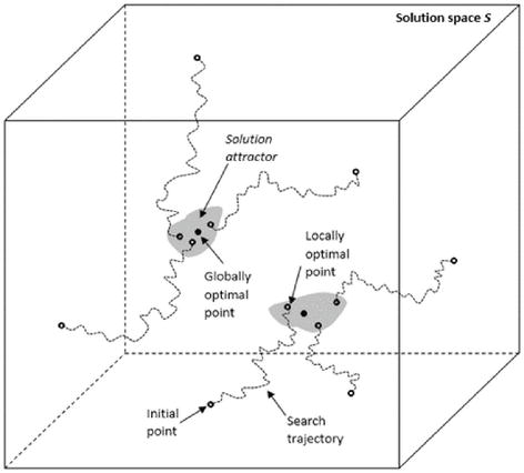
Figure 5.

Analogy of the concepts of serch trajectories and solution attractors in a local search system for a multimodal optimization problem.

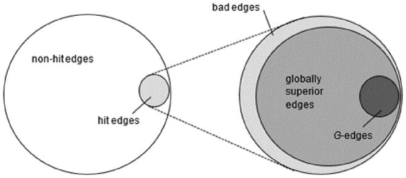
A search trajectory in a local search system changes its edge configuration during the search according to the objective function f southward and its neighborhood structure. The matrix E tin can follow the "footprints" of search trajectories to capture the dynamics of the local search system. When all search trajectories reach their end points – the locally optimal tours, the edge configuration of the matrix Eastward will become stock-still, which is the edge configuration of the solution attractor A . This fixed edge configuration contains two groups of edges: the edges that are not hit past whatever of locally optimal tours (non-striking edges) and the edges that are striking by at least one of the locally optimal tours (hitting edges). Effigy six shows the border grouping in the edge configuration of E when all search trajectories cease at their terminal points.

Figure 6.

The group of the edges inEwhen all search trajectories reach their end points.

In the ABSS, we use Thou search trajectories in the local search phase. Different sets of M search trajectories will generate dissimilar last border configuration of Due east . Suppose that, we kickoff the local search from a gear up of K initial points and obtain a border configuration Yard a in E when the local search phase is terminated. Then nosotros start the local search procedure again from a different set of K initial points and obtains a little dissimilar edge configuration M b in E . Which border configuration truly describes the border configuration of the real solution attractor? Actually, Grand a and Chiliad b are structurally equivalent because they are dissimilar only in the set of bad edges, thus Thousand a precisely replicates the dynamical backdrop of M b . The final edge configuration of the synthetic solution attractor generated from 1000 search trajectories is non sensitive to the selection of K search trajectories. This property indicates that a heuristic local search system really is a deterministic system: although a single search trajectory appears stochastic, all search trajectories from differeitn initial points will exist always trapped into the same modest region in the solution space and the terminal border configuration of E will always converge to the same set of the globally optimal edges.

The convergence of the search trajectories tin be measured by the change in the edge configuration of the matrix East . In the local search process, search trajectories collect all available topology information nigh the quality of the edges from their search experience and record such data in the matrix Due east . The changes in the edge configuration of E fully reflects the real search evolution of the search system. A state of convergence is achieved once no any more local search trajectory tin can change the border configuration of E . For a set of search trajectories to be converging, they must exist getting closer and closer to each other, that is, their edge configurations go increasingly similar. As a outcome, the edge configurations of the search trajectories converge to a small set of edges that contains all globally superior edges and some bad edges. Let W denote total number of edges in Eastward , α t the number of the edges that are hit by all search trajectories at time t , β t the number of the edges that are hit past one or some of the search trajectories, and γ t the number of edges that have no hit at all, then at any fourth dimension t , we have

For a given TSP instance, Due west is a abiding value W = n northward − i / 2 for a symmetric instance or West = n northward − 1 for an asymmetric instance. During the local search process, the values for α t and γ t will increase and the value for β t will decrease. However, these values cannot increase or decrease foreover. At certain point of time, they will become constant values, that is,

W = lim t → ∞ α t + lim t → ∞ β t + lim t → ∞ γ t = Α + B + Γ

E8

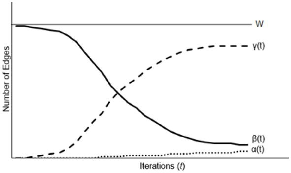
Our experiments confirmed this inference most α t , β t and γ t . Figure vii illustrates the patterns of α t , β t and γ t curves generated in our experiments. Our experiments besides establish that, for unimodal TSP instances, the ratio γ t / W could arroyo to 0.70 quickly for dissimilar sizes of TSP instances. For multimodal TSP instances, this ratio depends on the number of the globally optimal points. However, the ready of hit edges is still very small.

Effigy 7.

The α t , β t and γ t curves with search iterations.

In summary, we assume a TSP instance Q has a solution space with h ≥ 1 globally optimal tours ( s 1 ∗ , s 2 ∗ , … , due south h ∗ ), and correspondingly in that location be h set of M -edges G ane K 2 … Chiliad h . A local search organization for the Q will generate h solution attractors A one A two … A h that attract all search trajectories. The edge configuration of the solution attractor A is the marriage of the border configurations of the h solution attractors. The terminal edge configuration of E represents the border configuration of A with three properties:

1. Information technology contains all locally optimal tours;

2. Information technology contains a complete collection of solution attractors, i.due east. A = A ane ∪ A ii ∪ … ∪ A h ;

3. It contains a consummate collection of G -edges, i.e. G = G one ∪ Yard two ∪ … ∪ G h .

From this analysis, nosotros can meet that the edge matrix E is an extremely useful data structure that not just collcets the information well-nigh search trajectories, but also convert local search behavor of private search trajectories into global search behavor of the search system. The global convergence and deterministic property of the search trajectories make the local search system always converge to the aforementioned solution attractors and the edge configurations of the search trajectories always converge to the same set up of globally superior edges. The matrix E shows us conspicuously where the search trajectories go and where all locally optimal points are located. We found the village! However, information technology is withal difficult to place all One thousand -edges among the globally superior edges. The ABSS uses the exhaustive search phase to observe all tours in the solution attractor. Since the local search phase has significantly reduced the size of the search space for the exhaustive search stage, the consummate search in the solution attractor becomes feasible.

Advertisement

5. Global optimization characteristic of the ABSS

The chore of a global optimization arrangement is to discover all admittedly best solutions in the solution space. There are two major tasks performed by a global optimization system: (ane) finding all globally optimal points in the solution space and (two) making certain that they are globally optimal. So far we exercise not have any constructive and efficient global search algorithm to solve NP-hard combinatorial issues. We practise not even have well-developed theory or assay tool to assistance us design efficient algorithms to perform these two tasks. One critical question in global optimization is how to recognize the globally optimal solutions. Modern search algorithms lack applied criteria that decides when a locally optimal solution is a globally optimal ane. What is the necessary and sufficient condition for a feasible point southward i to be globally optimal point? The mathematical status for the TSP is ∀ south ∈ S , f s ∗ ≤ f south . To run across this condition, an efficient global search arrangement should take the following backdrop:

1. The search organisation should be globally convergent.

2. The search system should be deterministic and have a rigorous guarantee for finding all globally optimal solutions without excessive computational burden.

3. The optimality benchmark in the arrangement must exist based on information on the global behavior of the search system.

The ABSS combines beautifully two crucial aspects in search: exploration and exploitation. In the local search phase, G search trajectories explore the full solution infinite to identify the globally superior edges, which form the edge configuration of the solution attractor. These Chiliad search trajectories are independently and invidually executed, and therefore they create and maintain diverseness from showtime to the stop. The local search stage is a randomized process due to randomization in the local search role one thousand s . In this sense, the Grand search trajectories actually perform the Monte Carlo simulation to sample locally optimal tours. The essential idea of Monte Carlo method is using randomness to solve problems that might be deterministic in principle [26]. In the ABSS, K search trajectories kickoff a sample of initial points from a uniform distribution over the solution space S , and, through the randomized local search process, generate a sample of locally optimal points uniformly distributed in the solution attractor A . The edge configuration of E is actually constructed through this Monte Carlo sampling process.

Each of the K search trajectories passes through many neighborhoods on its fashion to the final point. For any tour s i , the size of North southward i is greater than n 2 ! [12]. Allow N due south i ′ announce the neighborhood of the terminal point s i ′ of the i ^th search trajectory and Ω Due north s tran i equally the marriage of the neighborhoods of all transition points of the search trajectory, and then we tin believe that the search infinite covered by Yard search trajectories is

N south i ′ ∪ ΩN south tran ane ∪ N s ii ′ ∪ ΩN southward tran 2 … ∪ N due south K ′ ∪ ΩN s tran K = S

E9

That is, the solution attractor A is formed through the entire solution space South . The solution attractor A contains h unique minimal "convex" sets A i i = 1 2 … h . Each A i has a unique best bout s i ∗ surrounded by a set of locally optimal tours. The tour s i ∗ in A i satisfies f southward i ∗ < f southward for all s ∈ A i and f s i ∗ = f southward 2 ∗ = … = f s h ∗ .

We see that the matrix E plays a disquisitional role to transform local search process of the private search trajectories into a collective global search process of the organisation. Each time when a local search trajectory finds a ameliorate tour and updates the edge configuraton of Due east , the provisional distribution on the edges are updated. More values are attached to the globally superior edges, and bad edges are discarded. Allow W be the complete ready of the edges in Eastward and W A the set of edges in the edge configuration of the solution attractor A such that g W is contained in the interior of Due west . Then the intersection Westward A of the nested sequence of sets is

and lim t → ∞ 1000 t Westward A = Due west A . As a result, the edge configurations of K search trajectories converge to a modest fix of edges.

The "convexity" property of the solution attractor A allows the propagation of the minimum property of s i ∗ in the solution attractor A i to the whole solution space S through the post-obit conditions:

1. ∀ s ∈ A i , f s i ∗ < f s

2. f s 1 ∗ = f s 2 ∗ = … = f southward h ∗

3. min s ∈ A f south = min s ∈ Due south f south

Therefore the global convergence and deterministic property of the search trajectories in the local search phase make the ABSS always find the same prepare of globally optimal tours. We conducted several experiments to ostend this argument empirically. In our experiments, for a given TSP instance, the ABSS performed the same search process on the instance several times, each fourth dimension using a unlike set of Grand search trajectories. The ABSS outputed the aforementioned set up of the best tours in all trials.

Table one shows the results of two experiments. One experiment generated due north = 1000 instance Q 1000 , the other generated northward = 10000 case Q 10000 . We conducted 10 trials on each of the instances respectively. In each trial, the ABSS used K = 6 due north search trajectories. Each search trajectory stopped when no improvement was made during 10 n iterations. The matrix East stored the edge configurations of the K final tours and so was searched completely using the depth-starting time tree search process. Table 1 lists the number of tours found in the synthetic solution attractor A , the cost range of these tours, and the number of the best tours constitute in the constructed solution attractor. For instance, in trial ane for Q chiliad , the ABSS found 6475824 tours with the cost range [3241, 4136] in the constructed solution attractor. There was a single best bout in the solution attractor. The ABSS found the aforementioned best tour in all x trials. For the instance Q 10000 , the ABSS plant the same prepare of four best tours in all 10 trials. These four all-time tours have the aforementioned cost value, but with different border configurations. If any trial had generated a unlike set of the best tours, nosotros could immediately brand a decision that the best tours in the constructed solution attractor may not be the globally optimal tours. From practical perspective, the fact that the aforementioned set of the best tours was detected in all trials provides an empirical bear witness of the global optimality of these tours. The fact also indicates that the ABSS converges in solution. Convergence in solution means that the search system can identify all optimal solutions repeatedly. E'er finding the same ready of optimal solutions actually is the fundamental requirement for global optimization systems.

Trial number	Number of tours in A	Range of tour cost	Number of best tours in A
Q thousand (6000 search trajectories)
ane	6475824	[3241, 4236]	1
ii	6509386	[3241, 3986]	1
3	6395678	[3241, 4027]	one
4	6477859	[3241, 4123]	1
5	6456239	[3241, 3980]	1
6	6457298	[3241, 3892]	1
seven	6399867	[3241, 4025]	one
8	6423189	[3241, 3924]	1
9	6500086	[3241, 3948]	1
10	6423181	[3241, 3867]	1
Q 10000 (60000 search trajectories)
1	8645248	[69718, 87623]	4
ii	8657129	[69718, 86453]	4
iii	8603242	[69718, 86875]	4
4	8625449	[69718, 87053]	4
v	8621594	[69718, 87129]	four
half-dozen	8650429	[69718, 86978]	4
seven	8624950	[69718, 86933]	4
eight	8679949	[69718, 86984]	iv
9	8679824	[69718, 87044]	iv
10	8677249	[69718, 87127]	four

Table 1.

Tours in constructed solution attractor A for Q g and Q 10000 .

Advertisement

6. Computing complexity of the ABSS

With current search applied science, the TSP is an infeasible problem because it is not solvable in a reasonable corporeality of time. Faster computers will not help. A feasible search algorithm for the TSP is one that comes with a guarantee to find all best tours in time at almost proportional to n thou for some power g . The ABSS can guarantee to detect all globally optimal tours for the TSP. Now the question is how efficient it is?

The cadre idea of the ABSS is that, if we have to use exhaustive search to confirm the globally optimal points, we should first detect a fashion to quickly reduce the effective search infinite for the exhaustive search. When a local search trajectory finds a better bout, we can say that the local search trajectory finds some meliorate edges. It is an inclusive view. Nosotros also can say that the local search trajectory discards some bad edges. Information technology is an sectional view. The ABSS uses the sectional strategy to conquer the TSP. The local search phase in the ABSS quickly prunes out large number of edges that cannot perchance be included in any of the globally optimal tours. Thus, a big useless area of the solution infinite is excluded. When the first edge is discarded by all K search trajectories, n − two ! tours that go through that edge are removed from the search space for the exhaustive search phase. Each time when an border is removed, large number of tours are removed from the search infinite. Although the complication of finding a truthful locally optimal tour is yet open, and nosotros even practise not know any nontrivial upper bounds on the number of iterations that may be needed to reach local optimality [27, 28], decades of empirical bear witness and applied inquiry have found that heuristic local search converges quickly, within depression guild polynomial time [1, 8, 27, 29]. In do, we are rarely able to find perfect locally optimal tour because we just practise non allow the local search procedure to run plenty long time. Ordinarily we let a local search process run a predefined number of iterations, accept whatever tour it generates, and treat it as a locally optimal bout. Therefore, the size of the constructed solution attractor depends not only on the problem structure and the neighborhood function, but also on the amount of search fourth dimension invested in the local search process. Equally nosotros increase local search fourth dimension, we volition constructe a smaller and stronger solution attractor. The local search stage in the ABSS can significantly reduce the search space for the exhaustive search stage by excluding a large number of edges. Usually the local search stage tin remove almost 60% of edges of the matrix Eastward in O n 2 .

Now an essential question is naturally raised: What is the human relationship between the size of the constructed solution attractor and the size of the problem instance? Unfortunately, at that place is no theoretical analysis tool bachelor in the literature that tin can be used to answer this question. Nosotros have to depend on empirical results to lend some insights. We conducted several experiments to discover the human relationship between the size of the constructed solution attractor and the TSP instance size. Figures viii–10 show the results of 1 of our experiments. All other like experiments reveal the same design. In this experiment, we generated 10 unimodal TSP instances in the size from k to 10000 nodes with grand-node increase. For each instance, the ABSS generated Grand = 6 n search trajectories. We first allow each search trajectory stop when no bout improvement was made during 10000 iterations regardless of the size of the instance (named "stock-still search time"). And so we did the aforementioned search procedures on these instances again. This time nosotros made each search trajectory end when no improvement was made during ten northward iterations (named "varied search time 1") and 100 due north iterations (named "varied search fourth dimension 2") respectively. Figure 8 shows the number of the edges that were discarded at the stop of local search phase. Figure 9 shows the number of tours in the constructed solution attractor for each instance, and Figure x shows the effective branching factors in the exhaustive search stage.

Figure 8.

The number of discarded edges at the terminate of local search phase.

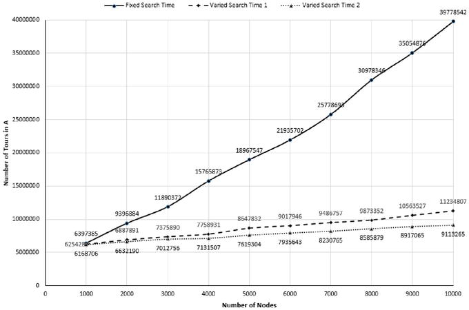
Figure ix.

Human relationship betwixt the size of the constructed solution attractor and instance size.

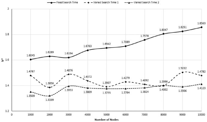
Figure 10.

The b ∗ values for unlike example sizenorthin our experiment.

In Figure 8, we can see that the search trajectories tin can speedily converge to a small set of edges. In the fixed-search-time example, about threescore% of the edges were discarded by search trajectories for the 1000-node case, but this percentage decreases equally instance size increases. For the 10000-node instance, just nigh 46% of the edges are discarded. However, if we increase the local search time linearly when the instance size increases, we can keep the aforementioned percentage of discarded-border for all instance sizes. In the varied-search-fourth dimension-1 case, about 60% of the edges are abandoned for all different instance sizes. In the varied-search-time-2 example, this percentage increases to 68% for all instances. College percentage of abandoned edges means that majority of the branches are removed from the search tree.

Figure 9 shows the number of tours be in the constructed solution attractor for these instances. All curves in the chart announced to exist linear relationship between the size of constructed solution attractor and the size of the problem instance, and the varied-search-time curves have much flatter slope because longer local search time makes a smaller constructed solution attractor. Figures 8 and 9 indicate that the search trajectories in the local search stage can effectively and efficiently reduce the search space for the exhaustive search, and the size of the solution attractor increases linearly as the size of the problem instance increases. Therefore, the local search phase in the ABSS is an efficiently asymptotical search process that produces an extremely modest search space for further exhaustive search.

The completely searching of the constructed solution attractor is delegated to the exhaustive search stage. This phase may still need to examine tens or hundreds of millions of tours simply nothing a computer processor cannot handle, equally opposed to the huge number of full possibilities in the solution infinite. The exhaustive search phase tin can find the exact globally optimal tours for the problem instance after a express number of search steps.

The exhaustive search phase can use any enumerative technique. Nevertheless, the border configuration of Eastward can be hands searched past the depth-first tree search algorithm. One of the advantages of depth-first tree search is less retentiveness requirement since just the nodes on the current path are stored. When using tree-search algorithm, nosotros normally apply branching factor, average branching gene, or effective branching factor to measure the computing complexity of the algorithm [xxx, 31, 32, 33]. In the information structure of search tree, the branching cistron is the number of successors generated by a given node. If this value is non uniform, an average branching gene can be calculated. An effective branching factor b ∗ is the number of sucessors generated by a typical node for a given tree-search problem. We use the following definition to calculate effective brancing factor b ∗ for the exhaustive search phase:

where due north is the size of the TSP instance, representing the depth of the tree, and N is total number of nodes generated in the tree from the origin node. In our experiments, the tree-search process e'er starts from node 1 (the commencement row of Due east ). Due north is full number of nodes that are candy to construct all valid tours and incomplete (therefore abandoned) tours in E . N does non count the node 1 (the origin node), but includes the node 1 as the end node of a valid tour. We use Figure 2(d) as an case. The depth-first search process searches the edge configuration of East and will generate N = 58 nodes. Therefore, b ∗ ≈ 1.3080 , that is, 58 ≈ i.3080 + 1.3080 2 + … + 1.3080 ten . Figure ten shows the constructive branching factor b ∗ in our experiment. The low values of b ∗ indicates that the edge configuration of the solution attractor represents a tree with extremely sparse branches, and the degree of sparseness does not changes every bit the trouble size increase if we linearly increase local search fourth dimension in the local search phase for a big instance. The search time in the exhaustive search phase is probably in O n 2 since the size of the constructed solution attractor might be linearly increased with the trouble size north and the number of edges in E is polynomially increased with the problem size. Our experiments shows that the ABSS tin can significantly reduce the computational complexity for the TSP and solve the TSP efficiently with global optimality guarantee.

Therefore, the ABSS is a uncomplicated algorithm that increases in computational difficulty polynomially with the size of the TSP. In the ABSS, the objective pursued by the local search phase is "chop-chop eliminating unnecessary search space every bit much every bit possible." It tin can provide an respond to the question "In which pocket-sized region of the solution infinite is the optimal solution located?" in time of O n 2 . The objective of the exhaustive search stage is "identifying the best tour in the remaining search infinite." It can provide an anwer to the question "Which is the best tour in this small region?" in time of O n two . All together, the ABSS can answer the question "Is this tour the best tour in the solution infinite?" in time of O n two . Therefore, the ABSS is probably with computing complication of O n 2 and memory space requirement of O n two . This suggests that the TSP might not be as complex as nosotros might have expected.

Advertisement

7. Conclusion

Advances in computational techniques on the decision of the global optimum for an optimization problem can have great impact on many scientific and engineering fields. Although both the TSP and heuristic local search algorithms have huge literature, there is still a variety of open problems. Numerous experts have made huge advance on the TSP inquiry, but two fundamental questions of the TSP remain essentially open: "How can we find the optimal tours in the solution space, and how practise we know they are optimal?"

The P-vs-NP problem is about how fast we tin search through a huge number of solutions in the solution infinite [34]. Exercise we ever need to explore all the possibilities of the problem to discover the optimal one? Really, the P-vs-NP trouble asks whether, in general, nosotros can find a method that completely searches only the region where the optimal points are located [34, 35, 36]. About people believe P ≠ NP because we have made little fundamental progress in the area of exhaustive search. Modernistic computers tin greatly speed up the search, but the extremely large solution space would even so crave geologic search fourth dimension to find the exact optimal solution on the fastest machines imaginable. A new bespeak of view is needed to meliorate our chapters to tackle these difficulty problems. This paper describe a new idea: using efficient local search process to effectively reduce the search infinite for exhaustive search. The concept of solution attractor in heuristic local search systems may modify the way we recall virtually both local search and exhaustive search. Heuristic local search is an efficient search system, while exhaustive search is an effective search organization. The central is how we combines these two systems into ane system beautifully to conquer the cardinal issues of the hard optimization problems. In the TSP case, the border matrix Due east , a problem-specific data structure, plays a disquisitional role of reducing the search space and transforming local search to global search.

The ABSS is designed for the TSP. Even so, the concepts and formulation behind the search algorithm can be used for any combinatorial optimization problem requiring the search of a node permutation in a graph.

References

1. 1. Applegate DL, Bixby RE, Chaátal 5, Cook WJ. The Traveling Salesman Problem: A Computational Study. Princeton: Princeton Academy Press; 2006
2. two. Papadimitriou CH, Steiglitz One thousand. Combinatorial Optimization: Algorithms and Complexity. New York: Dover Publications; 1998
3. iii. Papadimitriou CH, Steiglitz K. On the complication of local search for the traveling salesman trouble. SIAM Journal on Calculating. 1977:vi:76–83
4. 4. Gomey J. Stochastic global optimization algorithms: a systematic formal approach. Computer science. 2019:472:53–76
5. v. Korte B, Vygen J. Combinatorial Optimization: Theory and Algorithms. New York: Springer; 2007
6. 6. Rego C, Gamboa D, Glover F, Osterman C. Traveling salesman problem heuristics: leading methods, implementations and latest advances. European Journal of Operational Inquiry. 2011:211:427–411
7. 7. Zhigliavsky A, Zillinakas A. Stochastic Global Optimization. New York: Springer; 2008
8. 8. Aart E, Lenstra JK. Local Search in Combinatorial Optimization. Princeton: Princeton Academy Press; 2003
9. 9. Michalewicz Z, Fogel DB. How to Solve It: Modern Heuristics. Berlin: Springer; 2002
10. 10. Sahni S, Gonzales T. P-complete approximation problem. Journal of the ACM. 1976:23:555–565
11. 11. Sourlas N. Statistical mechanics and the traveling salesman problem. Europhysics Letters. 1986:2:919–923
12. 12. Savage SL. Some theoretical implications of local optimality. Mathematical Programming. 1976:10:354–366
13. 13. Shammon CE. A mathematical theory of communication. Bong System Technical Journal. 1948:27:379–423&623–656
14. 14. Alligood KT, Sauer TD, York JA. Anarchy: Introduction to Dynamical System. New York: Springer; 1997
15. xv. Auslander J, Bhatia NP, Seibert P. Attractors in dynamical systems. NASA Technical Report NASA-CR-59858; 1964
16. sixteen. Brin M, Stuck Grand. Introduction to Dynamical Systems. Cambridge: Cambridge University Printing
17. 17. Brown R. A Mod Introduction to Dynamical Systems. New York: Oxford Academy Press
18. xviii. Denes A, Makey K. Attractors and footing of dynamical systems. Electronic Journal of Qualitative Theory of Differential Equations. 2011:xx(20):one–eleven
19. 19. Fogedby H. On the phase space approach to complication. Periodical of Statistical Physics. 1992:69:411–425
20. xx. Milnor J. On the concept of attractor. Communications in Mathematical Physics. 1985:99(ii):177–195
21. 21. Milnor J. Collected Papers of John Milnor VI: Dynamical Systems (1953–2000). American Mathematical Society; 2010
22. 22. Ruelle D. Pocket-size random perturbations of dynamical systems and the definition of attractor. Communications in Mathematical Physics. 1981:82:137–151
23. 23. Li W. Dynamics of local search trajectory in traveling salesman problem. Journal of Heuristics. 2005:11:507–524
24. 24. Li W, Feng M. Solution attractor of local search in traveling salesman trouble: concepts, structure and application. International Journal of Metaheuristics. 2013:2(3):201–233
25. 25. Li Westward, Li X. Solution attractor of local search in traveling salesman problem: computational written report. International Periodical of Metaheuristics. 2019:7(2):93–126
26. 26. Kroese DP, Taimre T, Botev ZI. Handbook of Monte Carlo Methods. New York: John Wiley & Sons; 2011
27. 27. Fischer ST. A note on the complication of local search problems. Information Processing Letters. 1995:53(ii):69–75
28. 28. Chandra B, Karloff HJ, Tovey CA. New results on the old-opt algorithm for the traveling salesman problem. SIAM Periodical on Computing. 1999:28(6):1998–2029
29. 29. Grover, LK. Local search and the local construction of NP-complete problems. Operations Inquiry Messages. 1992:12(4):235–243
30. xxx. Baudet GM. On the branching factor of the alpha-beta pruning algorithm. Artificial Intelligence. 1978:10(23):173–199
31. 31. Edelkamp S, Korf RE. The branching factor of regular search space. Proceedings of the xv^th National Conference on Artificial Intelligence. 1998:292–304
32. 32. Korf RE. Depth-start iterative deepening: an optimal admissible tree search. Artificial Intelligence. 1985:27:97–109
33. 33. Pearl J. The solution for the branching gene of the alpha-beta pruning algorithm and its optimality. Advice of the ACM. 1982:25(eight):559–564
34. 34. Fortnow L. The Gilt Ticket – P, NP, and the Search for the Impossible. Princeton: Princeton University Press; 2013
35. 35. Fortnow L. The status of the P versus NP problem. Communication of the ACM. 2009:52(nine):78–86
36. 36. Sipser M. The history of status of the P verses NP question. Proceedings of 24^th Annual ACM Symposium on Theory of Computing. 1992:603–618

Submitted: September 23rd, 2020 Reviewed: Jan 20th, 2021 Published: February ninth, 2021

© 2021 The Author(due south). Licensee IntechOpen. This chapter is distributed under the terms of the Artistic Eatables Attribution 3.0 License, which permits unrestricted utilize, distribution, and reproduction in whatever medium, provided the original work is properly cited.

Source: https://www.intechopen.com/chapters/75156

Posted by: pageothessonce.blogspot.com

Share this post